Regression Module
Regression is a type of supervised learning used to predict a numeric outcome from one or more predictor variables (features).
There are two main types of regression methods:
1. Parametric Regression Parametric methods assume a specific mathematical form for the relationship between predictors and the outcome. The model has a fixed number of parameters that are estimated from the data. Example: Linear regression.
2. Nonparametric Regression Nonparametric methods do not assume a specific equation. Instead, they learn the relationship directly from the data, allowing for more flexible patterns but often requiring larger datasets. Example: K-nearest neighbors (KNN) regression.
0. Linear Regression (KNN)
In this module, we will focus on linear regression, a commonly used parametric regression method.
0.1 How Linear Regression works
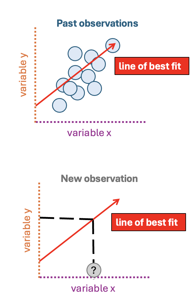
Linear regression is a statistical method used to model the relationship between a predictor variable and a numeric outcome. It works by finding the best-fitting straight line that summarizes the pattern in the data.
For example, if we collect data on how many hours students study and their exam scores, linear regression can draw a line that shows how study time is related to performance. This line captures the overall trend—students who study more tend to have higher scores—and allows us to predict the expected score for a given amount of study time.
It is called linear regression because the relationship between the variables is represented by a straight line.
The main idea is:
To predict the response variable for a new observation, linear regression finds patterns in a dataset of past observations and draws a line of best fit through the data.
Simple linear regression equation
The equation for the straight line is: \[ y = \beta_1 x + \beta_0 \] where:
\(y\) the response variable or the outcome you’re trying to predict.
\(x\) the predictor variable factor you’re using to make the prediction.
\(\beta_1\) the slope of the line; how much \(y\) changes per each unit change in \(x\).
\(\beta_0\) the y intercept; or the starting value of \(y\) when \(x\) is 0.
Using data to find the line of best fit means finding the coefficients \(\beta_1\) and \(\beta_0\), which define the line.
1. Load and inspect our data
Let’s begin by loading the libraries we need and importing our dataset.
In this module, we will demonstrate the analysis in both R and Python, so you can see how the same machine learning workflow is implemented in each language.
We will be working with the Body Fat Prediction dataset, an open-access dataset commonly used to illustrate regression techniques.
Each row in the dataset represents measurements from a single individual. The columns contain numerical measurements describing different body circumference features (such as neck, chest, abdomen, hip, and thigh).
Our target variable is Percent body fat, which represents the percentage of a person’s total body weight that is made up of fat tissue. The goal is to use a linear regression model to predict percent body fat using the other body measurement features in the dataset.
To get a quick look at the data, let’s display the first few rows of the dataset.
In Python,
We can use the .head() method to display the first few rows of a DataFrame.
In R,
We can use the head() function to view the first few rows of the dataset.
This helps us understand how the data is structured, what the column names are, and how the variables are formatted before beginning our analysis.
1.1 Assumptions before fitting our model
As a parametric method, linear regression makes specific assumptions about the data. Before fitting a model, it’s important to check these assumptions to ensure that the results are valid and interpretable.
1. Linearity: The relationship between the predictor(s) (X) and the response variable (Y) should be approximately linear.
How to check:
- Create a scatter plot of the predictor versus the response.
- If the points roughly form a straight-line pattern, the linearity assumption is likely satisfied.
- Deviations from a straight-line pattern may indicate that a linear model is not appropriate, or that a transformation of the variables is needed.
Let’s create a scatter plot to visualize the relationship between the predictor variable (abdomen circumference) on the x-axis and the response variable (body fat percentage) on the y-axis. This helps us see the overall trend in the data and whether a linear relationship exists between the two variables.
We can see that in this data set, larger abdomen circumference tend to have higher body fat percentage. This means we might be able to predict the body fat percentage of an individual based on their abdomen circumference!
Note: It’s important to remember that we’re not saying a larger abdomen circumference causes a higher body fat percentage; we’re just observing that larger abdomen circumference are generally associated with higher body fat, so abdomen circumference can help us estimate the percentage.
2. Independence: The data points should be independent, meaning the errors (residuals) of one observation should not be correlated with those of another.
How to think about it:
- In typical data sets with individual measurements (like body fat for different people), independence is usually reasonable because one person’s body fat does not affect another’s.
- If the data were collected over time or in clusters (e.g., repeated measurements from the same individual or family), the independence assumption might be violated.
- In such cases, you would need to check for autocorrelation or consider models that account for dependence, such as mixed-effects models.
3. No or Little Multicollinearity: In multiple linear regression, the predictor variables should not be highly correlated with each other.
Why it matters:
- High correlation between predictors makes it difficult for the model to separate out the individual effect of each predictor on the response.
- This can lead to unstable coefficient estimates and inflate standard errors, making it harder to interpret the results.
How to detect it:
- One common method is the Variance Inflation Factor (VIF).
- A high VIF indicates that a predictor is strongly correlated with other predictors in the model.
- If multicollinearity is detected, you may need to remove or combine correlated predictors.
When modeling just one predictor (simple linear regression), we don’t have to worry about this!
2. Data Processing
Now that we’ve loaded, and inspected our data, as well as checked model assumptions, the next step is data processing.
Fortunately, linear regression is relatively simple to implement because it requires little model tuning and minimal data preparation.
Unlike many classification algorithms, linear regression does not require hyper-parameter tuning (such as choosing the number of neighbors in KNN). Instead, the model directly estimates the coefficients that define the best-fitting line.
In addition, linear regression typically does not require standardizing or scaling predictor variables. While scaling can sometimes help with interpretation or numerical stability, the model can still be fit correctly using predictors in their original units. This makes linear regression a useful starting point for understanding relationships between variables!
2.1 Removing NA Values
Linear regression and many other machine learning models require complete data. Missing values (NA values) can cause errors when fitting the model or lead to unreliable predictions. Therefore, it is important to identify and handle missing values before training the model, typically by removing rows with missing data.
In Python,
We can remove rows with missing values using the dropna() method.
In R,
We can achieve the same using the na.omit() function.
2.2 Training and Testing
Before building our model, it’s important to follow a key principle in machine learning:
Never use the test data to train the model. Doing so would let the model “see” the answers in advance, making its performance seem better than it actually is.
To ensure an honest evaluation, we split the dataset into a training set and a test set:
- Training set (usually 50–95% of the data): Used to help the model learn patterns and relationships between the predictors and the outcome.
- Test set (the remaining 5–50%): Reserved for evaluating model performance on new, unseen data.
Think of it like predicting body fat from body measurements:
- The training set contains the measurements and body fat percentages we already know, which the model uses to learn how features like abdomen or hip circumference relate to body fat.
- The test set contains measurements the model hasn’t seen before. If the model can accurately predict body fat here, it shows it has truly learned the relationship rather than just memorizing the training data.
This process ensures that our regression model can generalize to new observations, which is the ultimate goal of predictive modeling.
In practice, a 75/25 or 80/20 split is common. For our example, we’ll use 75% for training and 25% for testing, giving the model enough data to learn while keeping a reliable test set to measure performance.
In Python,
We can use train_test_split from scikit-learn to split the data.
Important parameters:
- random_state: sets a seed for reproducibility
- train_size: the proportion of data to include in the training set (0.75, meaning 75% of our data will be used for training, the remaining 25% for testing)
In R,
We can achieve the same using the createDataPartition() function from caret.
Important parameters:
df$BodyFat: preserves the distribution of the target variable (BodyFat) - p: the proportion of data to include in the training set (0.75, meaning 75% of our data will be used for training, the remaining 25% for testing) - list: whether to return indices as a list (FALSE returns a vector, which is easier to use for subsetting)
3. Implementing Simple linear regression
Now that our data is cleaned, and split into training and testing sets, we are ready to move on to building our linear regression model.
3.1 Fit the linear regression model on the train set
This means that, according to our linear regression model, for every additional inch in abdomen circumference, body fat percentage increases by our slope value.
The model also estimates a negative intercept value, meaning that when abdomen circumference is 0, the predicted body fat percentage would be negative. While this doesn’t make intuitive or physiological sense (nobody has a 0-inch abdomen), the intercept is simply a mathematical starting point for the line—it helps define the position of the regression line in the coordinate system.
Note: It’s common to see slightly different coefficients (slopes and intercepts) between Python and R, even when using the same data and train/test split. This is usually due to minor differences in numerical precision, or data handling. These differences are very small and do not affect the overall pattern or predictions—both models are essentially fitting the same line of best fit.
3.2 Assumptions after fitting our model
Once you’ve fitted your regression model, it’s important to check a few additional assumptions. These assumptions ensure that the model is reliable.
4. Homoscedasticity: The spread of the residuals (errors) should be roughly constant across all values of the predictor(s).
How to check:
- Plot the residuals vs. fitted values (predicted Y).
- If the residuals are evenly spread around zero with no clear pattern or “funnel shape,” the assumption of homoscedasticity is satisfied.
- Uneven spread indicates heteroscedasticity, which can affect the accuracy of coefficient estimates and their standard errors.
In Python,
To check homoscedasticity, we can plot the model’s predicted values against the residuals (errors).
In R,
This is made very simple using diagnostic plots directly from the model object! The first plot (which = 1) shows residuals vs fitted values.
5. Normality of Errors: The residuals should be approximately normally distributed.
Why it matters:
- Normality of errors is important for valid hypothesis testing and confidence intervals on regression coefficients.
How to check:
- Use a Q-Q plot of the residuals. This plots the distribution of our residuals against the theoretical normal distribution.
- If the points lie roughly along a straight diagonal line, the residuals are approximately normal.
- Small deviations are usually not a major problem, especially with large data sets.
In Python,
To check normality of residuals, we can use the qqplot function from the statsmodels package.
In R,
This is made very simple using diagnostic plots directly from the model object! The second plot (which = 2) shows normality of residuals.
By checking these assumptions, you can be confident that your regression model provides trustworthy predictions and that statistical tests based on the model are valid.
3.3 Model evaluation
Now that we’ve determined our model’s assumptions are met, let’s move on to evaluation.
Unlike classification, where we measure accuracy by how often predictions match the true labels, regression predictions rarely match the exact values of the response variable. Instead, we evaluate regression models using metrics such as Root Mean Square Prediction Error (RMSPE) and R-squared (coefficient of determination).
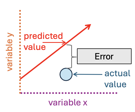
- RMSPE tells us how far off our predictions are on average. A smaller RMSPE means the model’s predictions are closer to the actual values, indicating better predictive accuracy.
- R-squared measures how well the model explains the variability in the response variable. It represents the proportion of variance in the response that is accounted for by the predictor(s). R-squared values range from 0 to 1, with values closer to 1 indicating that the model explains more of the variation in the outcome.
Together, these metrics provide a comprehensive view of model performance: R-squared shows how well the model fits the data, while RMSPE reflects the accuracy of predictions on new, unseen data.
In Python,
To evaluate performance on the test set, we use the predict() method to generate predicted values and then compare them to the true values using functions like mean_squared_error() for RMSPE and r2_score() for R-squared.
In R,
We similarly use the predict() function in R to generate predictions on the test set and then compare them to the actual values to calculate RMSPE and R-squared. However, unlike Python, R does not provide built-in functions to compute these metrics on new data, so we calculate them manually using basic arithmetic and summary statistics. This involves taking the differences between predicted and actual values to compute RMSPE, and calculating the proportion of variance explained for R-squared.
Our final model’s test error, measured by RMSPE, tells us how far off our predictions are on average, in body fat percentage units.
The coefficient of determination (R-squared) shows how well the model explains the variability in body fat based on abdomen circumference. A higher R-squared means that a larger proportion of the variation in body fat is captured by the model, indicating a strong relationship between the predictor and the outcome.
4. Implementing multiple linear regression
4.1 Fitting the multiple linear regression model on the train set
If we want to include another predictor in our model, we simply expand the equation to account for multiple predictors:
\[ y = \beta_0 + \beta_1 x_1 + \beta_2 x_2 \]
Where:
- \(y\) is the response variable (body fat percentage)
- \(x_1, x_2\) are the predictor variables (e.g., abdomen circumference, hip circumference)
- \(\beta_0\) is the intercept
- \(\beta_1, \beta_2\) are the slopes, showing how much (y) changes per unit change in each predictor
This is the basis of multiple linear regression, where the model can learn relationships between the outcome and several predictors at once!
For example, if we wanted to examine how abdomen and hip circumference are associated with body fat percentage, we would use multiple linear regression to include both predictors in the model.
In Python,
We include both columns in the predictor set:
In R,
We include both predictors in the formula using +
Here, the intercept represents the predicted body fat percentage when both abdomen and hip circumferences are zero. While this may not be physically meaningful, it serves as the starting point of the regression plane.
The slope for Abdomen represents the change in body fat percentage for every one-unit increase in abdomen circumference, holding hip circumference constant.
Similarly, the slope for Hip represents the change in body fat percentage for every one-unit increase in hip circumference, holding abdomen circumference constant.
In multiple linear regression, the intercept and slopes together define the regression plane that models the relationship between the predictors and the outcome.
4.2 Assumption of multicolinearity
It’s important to check that these variables are not highly collinear, as multicollinearity can violate the assumptions of our regression model.
In Python,
We can use the variance_inflation_factor() function from the statsmodels package.
Important things to consider: add_constant adds the intercept term, which is required for correct VIF calculation. The first row (const) will usually have a very high VIF — you can ignore that; focus on your predictors (Abdomen, Hip).
In R,
We use the vif function from the car package. R automatically handles the constant/intercept, so you don’t need to add it manually.
Note. VIF >/ 10 signals strong multicollinearity.
We can also confirm homoscedasticity and normality of errors.
4.3 Model evaluation
Now that we’ve determined our model’s assumptions are met, we can move on to evaluation.
These steps are very similar to what we did with simple linear regression: we calculate prediction error (e.g., RMSPE) and R-squared to assess how well our model fits the data.
The only difference in multiple linear regression is that we also want to consider Adjusted R-squared.
Why Adjusted R-squared ? In multiple regression, adding more predictors to the model will always increase R-squared, even if those predictors do not meaningfully improve the model.Adjusted R-squared corrects for this by penalizing unnecessary predictors. It accounts for both the number of predictors (p) and the sample size (n). This provides a more honest measure of model fit: a higher Adjusted R-squared indicates that the predictors collectively explain variance in the outcome beyond what would be expected by chance.
Our final model’s test error, measured by RMSPE, tells us how far off our predictions are on average, in body fat percentage units.
The coefficient of determination (R-squared) shows how well the model explains the variability in body fat based on abdomen and hip circumference. A higher R-squared means that a larger proportion of the variation in body fat is captured by the model, indicating a strong relationship between the predictors and the outcome.
5. Overview of Linear Regression Workflow
That’s it! In this module, we explored how predictors like Abdomen and Hip circumference relate to body fat percentage using simple and multiple linear regression and assessed the model’s assumptions and fit. Here’s a summary of the linear regression workflow:
Select Predictors and Outcome
- Choose the variables to include in the model (e.g.,
AbdomenandHipas predictors,Body Fat %as the outcome). - Split the dataset into training and test sets to evaluate model performance on unseen data.
- Choose the variables to include in the model (e.g.,
Fit the Linear Regression Model
- Use simple or multiple linear regression to estimate the coefficients (slopes and intercept).
Check Model Assumptions
- Linearity: The relationship between predictors and the outcome should be approximately linear.
- Independence: Observations should be independent of each other.
- Homoscedasticity: Residuals should have constant variance across all predicted values.
- Normality of Residuals: Residuals should be approximately normally distributed.
- Multicollinearity: Predictors should not be highly correlated (check VIF in multiple regression).
Interpret Coefficients
- Each slope represents the change in the outcome for a one-unit change in the predictor, holding other predictors constant.
- The intercept represents the predicted outcome when all predictors are zero (mathematical reference point).
Evaluate Model Performance
- Use metrics like RMSPE (Root Mean Square Prediction Error) to assess prediction accuracy.
- Use R-squared and Adjusted R-squared to evaluate how well the model explains variance in the outcome.