Classification Part 1 Module
Classification is a type of supervised learning where we use one or more predictor variables (features) to predict a categorical outcome (also called a class label).
Instead of predicting a continuous number (like in regression), classification predicts which category an observation belongs to.
Types of Classification
Binary classification: The outcome has two possible categories. Example: Diagnosing a patient as disease vs healthy.
Multiclass classification: The outcome has more than two categories. Example: Classifying a patient’s condition as major depressive disorder, bipolar disorder, or schizophrenia spectrum disorder based on clinical or biological features.
0. K-nearest neighbors (KNN)
In this module, we will focus on K-nearest neighbors (KNN), a widely used classification algorithm. While KNN is the primary method covered here, many other classification approaches exist (see Classification Part 2 module).
0.1 How KNN works
K-Nearest Neighbors (KNN) is a simple and intuitive classification method.
The main idea is:
To predict the label of a new observation, KNN looks at the most similar observations in the training dataset and lets them “vote.”
Step 1: Measure Similarity
To determine which observations are most similar (or “closest”), KNN calculates the distance between data points.
Most commonly, this is the straight-line distance between points (also called Euclidean distance).
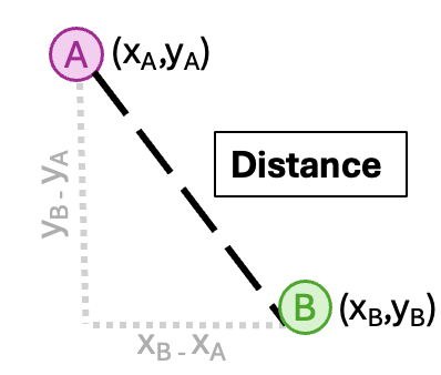
Observations that are closer together are considered more similar.
Step 2: Choose K
K is a number we choose ahead of time, we call this a hyper-parameter. It represents how many neighbors we will consider when making a prediction.
For example:
If K = 1, the algorithm looks at the 1 closest observation.
If K = 5, it looks at the 5 closest observations.
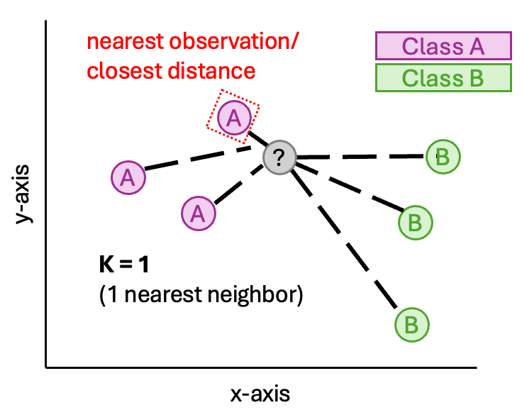
The new observation is then assigned the class that appears most often among those K neighbors.
0.2 But wait! How do we choose K?
Choosing the right value of K is important.
What if K is too small?
If we choose K = 1, for example, the new observation is assigned the class of the single closest data point.
This can be risky.
If that closest point happens to be an outlier (an unusual or extreme observation), the prediction may not reflect the overall pattern in the data. In this case, the model becomes too sensitive to noise.
For example, imagine you want to guess how many hours your classmates sleep each night. Most sleep around 7–8 hours, but one friend slept only 2 hours last night because they pulled an all-nighter. If you use that friend’s sleep as the ‘closest example,’ your prediction would be way too low and wouldn’t reflect the usual sleep pattern of the class.
What if K is too large?
On the other hand, if we choose a very large K — for example, K equal to the total sample size — the classifier would consider all observations when making a prediction.
Taking the same example, if you take the average of everyone in the class (including night owls and early risers), your prediction would be very smooth and stable, but it might ignore the specific habits of students most similar to the person you’re predicting for.
This would make the model too simple. It would ignore local patterns and tend to predict the majority class most of the time.
In this case, the model fails to capture meaningful structure in the data.
The Key Idea
Small K: very flexible, sensitive to noise (risk of overfitting)
Large K: very simple, may miss important patterns (risk of underfitting)
In practice, we choose K carefully (often using cross-validation, which we will talk about) to balance these two extremes.
1. Load and inspect our data
Let’s begin by loading the libraries we need and importing our dataset.
In this module, we will demonstrate the analysis in both R and Python, so you can see how the same machine learning workflow is implemented in each language.
We will be working with the Wisconsin Diagnostic Breast Cancer (WDBC) dataset. This dataset is commonly used in machine learning classification tasks and contains several features computed from digitized images of breast tumor cells.
Each row in the dataset represents a single tumor. The columns contain numerical measurements describing characteristics of the cell nuclei (such as radius, texture, perimeter, and area).
Our target variable is Diagnosis, which indicates whether the tumor is malignant or benign. Our goal will be to build a KNN classifier to predict the diagnosis using the other features in the dataset.
To get a quick look at the data, let’s display the first few rows of the dataset.
In Python,
We can use the .head() method to display the first few rows of a DataFrame.
In R,
We can use the head() function to view the first few rows of the dataset.
This helps us understand how the data is structured, what the column names are, and how the variables are formatted before beginning our analysis.
To better understand our target variable, we can examine the unique classes in the Diagnosis column.
In both Python and R, we can check the distinct values present in this column to see which categories we are trying to predict. This allows us to confirm whether the problem is binary or multiclass and to understand how the outcome variable is coded in the dataset.
In Python,
We can use the .unique() method in pandas to return the distinct values in a column.
In R,
We can use the unique() function to achieve the same result.
2. Data Processing
Now that we’ve loaded and inspected our data, the next step is data processing.
2.1 Removing NA values
KNN and many other machine learning models rely on complete data. Missing values can cause errors or inaccurate predictions, so it’s important to handle them before building the model!
In Python,
We can remove rows with missing values using the dropna() method.
In R,
We can achieve the same using the na.omit() function.
By ensuring the dataset contains complete cases only, we prepare it for subsequent steps like feature scaling and training the KNN classifier.
2.2 Standardization
One important part of preprocessing for KNN is standardizing the features so that all variables are on the same scale.
Why is this important? KNN relies on distance calculations to find the nearest neighbors. If one feature has much larger values than others, it can dominate the distance metric and bias the model!
For example, suppose you want to use KNN to predict a student’s exam performance based on hours studied (0–50 hours) and family income (in dollars, say 20,000–200,000). Without standardizing, the income values are much larger and dominate the distance calculation, so the model barely considers hours studied! By standardizing both features to the same scale, KNN treats each feature equally, so predictions better reflect both study time and income.
In Python,
We can use the StandardScaler() function from the sklearn.preprocessing module to standardize features. This transforms each feature so that it has a mean of 0 and a standard deviation of 1, ensuring that all features contribute equally to the distance calculations.
Explanation of steps:
Select columns. Decide which numeric features need standardization. For example, some columns like ID or diagnosis should not be scaled because they are identifiers or categorical labels. We can exclude them and then use the
DataFrame.columns.difference()method to select all remaining numeric columns for standardization.Initialize StandardScaler(). This creates a scaler object that knows how to standardize features.
Fit and transform. The
fit_transform()method computes the mean and standard deviation for each selected column and scales the data accordingly.Replace or save scaled features. You can overwrite the original columns in your DataFrame or store the scaled features in a new DataFrame for clarity.
In R,
We can achieve the same effect using the scale() function, which also centers and scales the features in a similar way.
Explanation of steps:
Select columns. Decide which numeric features need standardization. For example, some columns like ID or diagnosis should not be scaled because they are identifiers or categorical labels. We can exclude them and then use the
setdiff()function to select all remaining numeric columns for standardization.Standardize features. The
scale()function subtracts the mean and divides by the standard deviation for each selected column. This ensures that all numeric features contribute equally to distance-based algorithms like KNN.
Standardizing features is a crucial step in preparing data for distance-based classification algorithms like KNN.
2.3 Training and testing
Before we build our model, it’s important to remember a golden rule of machine learning:
You cannot use the test data to train the model! Doing so would let the model “see” the answers in advance, making it appear more accurate than it really is.
Imagine the consequences if a model incorrectly predicts that a patient’s tumor is benign when it’s actually malignant. Overestimating accuracy could lead to serious mistakes like this!
To avoid this, we split the data into a training set and a test set:
The training set (typically 50–95% of the data) is used to help the model learn patterns and relationships.
The test set (the remaining 5–50%) is reserved for evaluating how well the model performs on new, unseen data.
Think of it like preparing a doctor for an exam:
The training set is the practice cases—they learn to recognize patterns in tumors.
The test set is the actual exam—new cases they haven’t seen before. Performing well on the test shows they truly understand the task rather than just memorizing examples.
In practice, a 75/25 or 80/20 split is common. For our example, we’ll use 75% for training and 25% for testing, giving the model enough data to learn while keeping a reliable test set to measure performance.
In Python,
We can use train_test_split from scikit-learn to split the data.
Important parameters:
- random_state: sets a seed for reproducibility. This ensures that any operation involving randomness (like splitting data) produces the same results every time, making your analysis reproducible.
- train_size: the proportion of data to include in the training set (0.75, meaning 75% of our data will be used for training, the remaining 25% for testing)
- stratify: this ensures both training and test sets maintain the same proportion of malignant and benign cases as the original dataset.
In R,
We can achieve the same using the createDataPartition() function from caret.
Important parameters:
- df$diagnosis: similar to
stratify=df["diagnosis"]in Python, this preserves the proportion of each diagnosis category in the training and test sets, ensuring a stratified split that reflects the original distribution. - p: the proportion of data to include in the training set (0.75, meaning 75% of our data will be used for training, the remaining 25% for testing)
- list: whether to return indices as a list (FALSE returns a vector, which is easier to use for subsetting)
3. Implementing KNN
Now that our data is cleaned, standardized, and split into training and testing sets, we are ready to move on to building our KNN classifier.
Reminder: One key decision in KNN is choosing the value of K, the number of neighbors the algorithm considers when making a prediction.
To select the best K, we can use cross-validation.
3.1 Finding the best value of K via cross-validation
Cross-validation is a way to test how well our model works on new data while using only the training set.
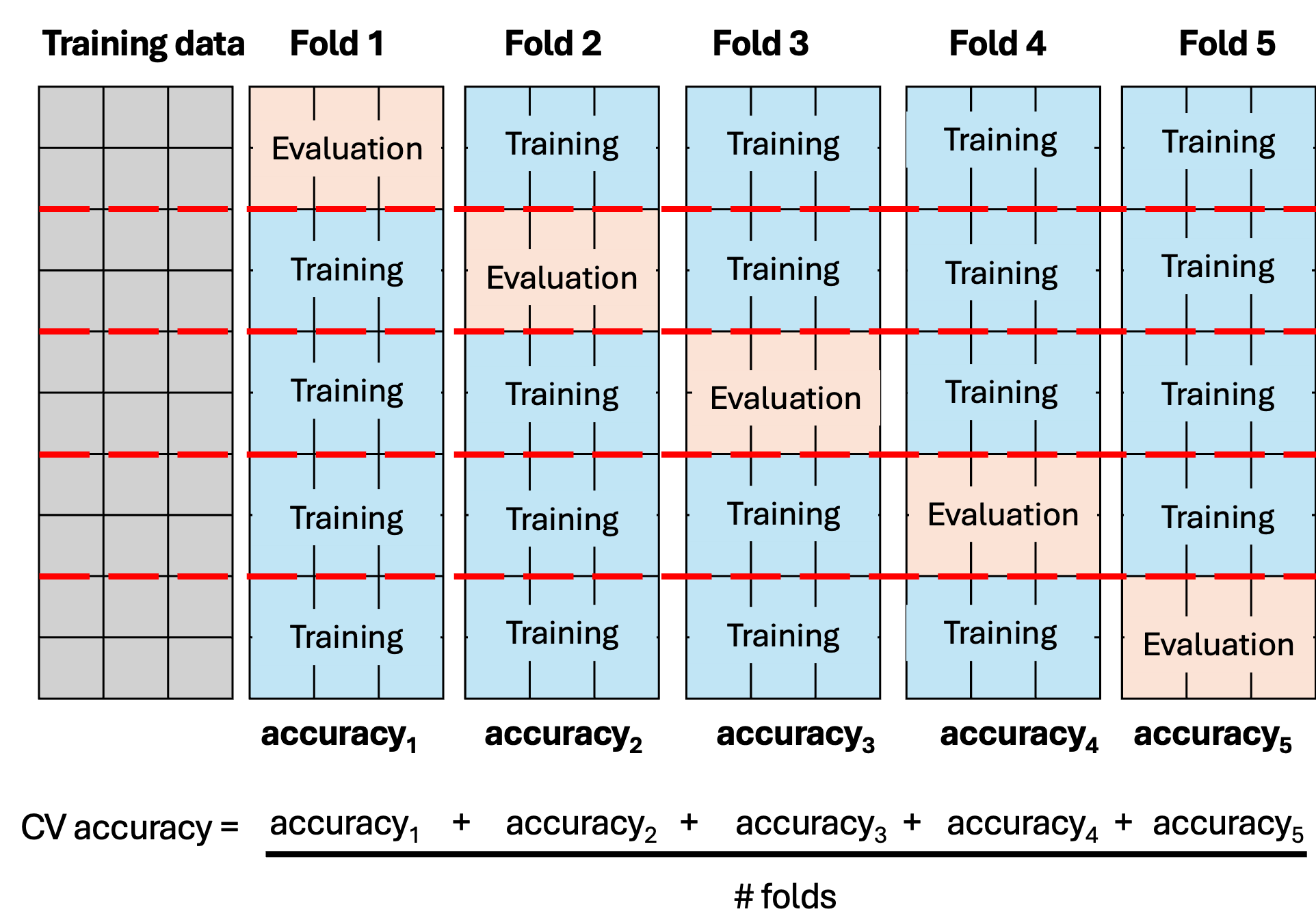
Instead of evaluating the model on a single split of the data, cross-validation creates multiple mini-classifiers by dividing the training data into several parts called folds.
Each fold gets a turn as the evaluation set, while the remaining folds are used to train the model.
This process is repeated until every observation has been used for evaluation exactly once and for training in the other folds.
The performance is then averaged across all folds to determine the best parameter value (e.g., the optimal K in KNN).
Why is this important? If we only used a single train-test split, our results could be misleading. We might get lucky or unlucky depending on which data points ended up in the training or evaluation sets. Cross-validation reduces this risk and gives a more reliable estimate of model performance.
One simple way to summarize a classifier’s performance is with accuracy.
Accuracy tells us the proportion of predictions that the model got right:
\[ \text{Prediction Accuracy} = \frac{\text{Number of correct predictions}}{\text{Total number of predictions}} \] A higher accuracy means the model is correctly predicting more cases.
Accuracy is easy to understand and gives a single number to evaluate how well the classifier is performing.
Note: Accuracy works well when the classes are fairly balanced. However, imagine a test for a rare disease that only 2 out of 100 people have. If the model predicts everyone is healthy, it’s 98% accurate—but it misses all the sick people. For highly imbalanced data, other metrics like precision, recall, or F1-score show how well the model detects the rare cases, unlike accuracy.
In Python,
GridSearchCV is a function in scikit-learn that automates hyperparameter tuning.
It works by trying a grid of values for the parameter you want to optimize (in this case, K).
For each K, it uses cross-validation on the training data to evaluate how well the model predicts unseen examples.
Finally, it selects the K that achieves the highest average accuracy across all folds.
In short, GridSearchCV systematically tests multiple K values and tells us which one works best for our dataset.
Now you may be asking, how do we know what range of K we should test? And unfortunately, the answer is— we don’t! This range is based on intuition. The goal is to explore a sufficiently broad range to cover the possibilities while staying practical and limiting computational load.
In R,
The train() function from the caret package can do the same thing in R.
You provide it with a model type (method = “knn”), the training data, and a tuning grid of K values to test.
It then performs cross-validation internally, evaluating each K by how accurately the model predicts on the held-out fold.
Finally, it chooses the K that maximizes accuracy.
Just like GridSearchCV in Python, train() automates the search for the best K and helps ensure that the value chosen generalizes well to new, unseen data.
Note: Small differences in the “best K” between Python and R can occur due to how ties are broken or internal implementation details in the KNN algorithm. The test set accuracy is often very similar even if the selected K differs.
Here we identified K = 16 as optimal, meaning each prediction uses the 16 nearest neighbors. We used only two features here for illustrative purposes but often times in real data analysis, more features would likely be included, which could improve performance but would require careful scaling and possibly a different K.
3.2 Model evaluation
To evaluate how well our model predicts unseen data, we check its accuracy on the test set.
We will use our KNN model found during cross-validation with the best K.
In Python,
When using GridSearchCV, this is automatic. Once GridSearchCV finds the best K, it refits the model on the full training set using that K. We can then evaluate the model on the test set by passing the test features and labels to the score() method.
In R,
With train(), we also refit the model automatically on the full training set using the best K. To evaluate accuracy on the test set, we use the predict() function to get predictions and then compare them to the true labels.
A test accuracy of 0.93 means the model correctly predicted the outcome for 93% of the observations in the test set. This suggests the model is performing well on new, unseen data!
4. Overview of KNN Workflow
That’s it! In this module, we classified tumors as benign or malignant using the Wisconsin Diagnostic Breast Cancer dataset and evaluated the model’s performance. Here’s a summary of the KNN workflow after data cleaning and preprocessing:
Define the Parameter Grid
- Specify the range of K values to test for tuning the KNN model.
Perform Grid Search
- Use
GridSearchCV(Python) ortrain()from caret (R) with the parameter grid to estimate the model’s accuracy for each K.
- Use
Execute Grid Search
- Fit the grid search instance to the training data to find the K that maximizes cross-validated accuracy.
Select Optimal K and Retrain the Model
- Retain the KNN model using the best K and fit it to the full training set.
- Both R (
train()) and Python (GridSearchCV) perform this automatically after tuning.
Evaluate the Model
Assess performance on the test set using:
score()in Pythonmean(predictions == true_labels)in R
This provides the final accuracy on unseen data.