Classification Part 2 Module
As a reminder, classification is a type of supervised learning where one or more predictor variables (features) are used to predict a categorical outcome (also called a class label).
0. Tree-Based Methods
This section builds on the Classification Part 1 module, focusing on tree-based methods.
0.1 How Tree-Based Methods Work
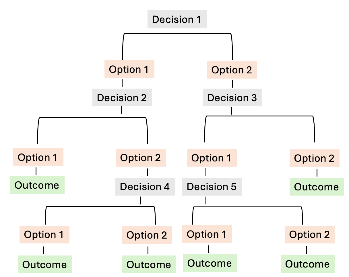
Tree-based methods are intuitive and visual. They make predictions by splitting data into groups based on the values of predictor variables (features).
Step-by-step process:
- Split the data into “boxes”
- Use a feature to divide the data.
- Each “box” contains points with similar feature values.
- Use a feature to divide the data.
- Make predictions within each box
- All points inside a box get the same prediction
- An observation is assigned to the class that is most frequent
Key point: Trees make decisions by splitting the data into groups where the observations are mostly similar. At each step, the tree picks a simple rule (like age < 40?) that best separates the data into these groups. This continues until each group is as uniform as possible, making it easier to make accurate predictions.
- For example, let’s say we want to predict whether a tumor will be benign or malignant
- The tree may split on features like perimeter, smoothness, or concavity.
- A final region might contain mostly “Benign” responses → New tumor falling in that region are classified as “Benign”
These splits form a tree-like structure, which is why we call them decision trees.
0.2 Tree Terminology 🌳
- Root / Internal Nodes: Points where data is split based on a rule (e.g., Age < 45).
- Branches: Lines connecting nodes that represent possible outcomes of a split.
- Leaves / Terminal Nodes: Groups at the bottom of the tree.
- Each leaf gives the predicted value, the most common category of the observations in that leaf.
0.3 Random Forest
Single decision trees are easy to understand but can be unstable.
- For example, two trees trained on slightly different data can give very different predictions.
We can improve this by combining many decision trees into one stronger model.
- This approach is called a Random Forest
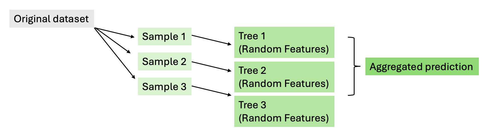
A Random Forest is like a team of decision trees working together to make better predictions.
- Each tree is built using a random sample of the data.
- At each split, the tree only looks at a random subset of features, so every tree is a little different.
- To make a prediction, each tree “votes,” and the majority vote wins
1. Load and inspect our data
We’re going to continue working with the Wisconsin Diagnostic Breast Cancer (WDBC) dataset. As a reminder, this dataset contains several features computed from digitized images of breast tumor cells.
Each row in the dataset represents a single tumor. The columns contain numerical measurements describing characteristics of the cell nuclei (such as radius, texture, perimeter, and area).
Our target variable is Diagnosis, which indicates whether the tumor is malignant or benign. Our goal will be to build a tree-based classifier to predict the diagnosis using the other features in the dataset.
Let’s start by loading the libraries, importing the dataset, cleaning it, and splitting it into training and testing sets.
Note: Unlike some algorithms (e.g., KNN), tree-based models do not require feature scaling, because each feature is considered independently when splitting the data.
For a refresher, see the Classification Part 1 Module.
2. Implementing Tree-based models
Now that our data is cleaned, standardized, and split into training and testing sets, we are ready to move on to building our tree-based classifier.
2.1 Decision Tree
Step 1. First, we define our features and target variable. Here, we are selecting all columns except diagnosis and id as predictor variables (X_train) and set the diagnosis column as the target (y_train). The target is converted to a categorical variable type so the model treats it as a classification problem. The same is done for the test set.
Step 2. Then we fit the model on the training data so it can learn the patterns.
In Python,
We create a decision tree using DecisionTreeClassifier() from scikit-learn.
In R,
We use the rpart() function from the rpart package with method = "class" to build a classification tree.
Step 3. Finally, we evaluate the model on the test set to see how well it predicts new data.
In Python,
We use the score() method on the test set to calculate accuracy. This tells us how well the model predicts new, unseen data.
In R,
We use the predict() function on the test set to generate predicted classes, then calculate the proportion of correct predictions to get the test accuracy.
Note: Small differences in accuracy between Python and R may occur; however, the results are generally very similar.
A test accuracy of 0.92 (Python) or 0.95 (R) means the model correctly predicted the outcome for 92%, or 95% of the observations in the test set. This suggests the model is performing well on new, unseen data!
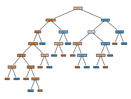
We can visualize these decision trees to see how the model makes decisions.
- Each internal node shows a feature and a rule
- Branches represent the possible outcomes of that rule.
- Leaves show the predicted class for that group of observations.
Visualizing the tree helps us interpret the model’s decision-making process, identify which features are most important, and see how combinations of feature values lead to different predictions. This makes the abstract concept of decision trees more concrete and intuitive.
In Python,
We can use plot_tree() from sklearn. Note, in browser-based Python, plot_tree() cannot render. We show a text-based tree here for learning, and include a visual example as a figure.
In R,
we can use rpart.plot()
Feature Importance
Instead of examining the entire tree, we can look at feature importance to understand which variables were most useful for making predictions.
- Feature importance scores range from 0 to 1
- A value close to 0 means the feature was rarely used by the model
- A value closer to 1 means the feature was very important for predicting the outcome
- All feature importance scores sum to 1
This helps us identify which features play the biggest role in predicting the target variable.
We can also visualize feature importance to easily compare which variables matter most.
In Python,
We can access feature importance using the feature_importances_ attribute from the trained decision tree model and visualize it with a bar plot.
In R,
Feature importance can be accessed from the variable.importance component of the rpart model and visualized using ggplot2.
Note. Because Python (sklearn) and R (rpart) implement decision trees slightly differently, the exact feature importance values may vary between the two languages. However, the most important predictors are usually similar.
Advantages and Limitations of Decision Trees
Decision trees have several advantages over many other algorithms:
- They are easy to visualize and interpret, especially when the trees are small. This makes them useful for explaining model decisions to non-experts.
- They are not sensitive to feature scaling. Because trees split on one feature at a time using simple threshold rules (e.g., radius < 15), the scale of the variables does not affect the model. This means we do not need to normalize or standardize the data before training a decision tree.
However, decision trees also have an important limitation:
- They can overfit the training data. A deep tree may learn patterns that are very specific to the training dataset rather than general patterns in the population. As a result, the model may perform well on the training data but poorly on new, unseen data.
Because of this limitation, methods such as ensemble approaches like random forests are often used to improve performance!
2.2 Random Forest
A random forest is a group of decision trees that work together to make predictions. Each tree is trained on a random sample of the data, and at each split it only considers a random subset of features. When predicting, each tree votes, and the majority vote decides the final class. This approach reduces overfitting and usually performs better than a single decision tree.
In Python,
We use RandomForestClassifier() from scikit-learn to build a random forest model. The process is similar to what we did with decision trees: we define the features and target variable, fit the model on the training data, and then evaluate its performance on the test data.
In R,
We use the randomForest()from the randomForest package to build a random forest model. Similar to Python, we train the model on the training data, then use it to make predictions on the test data and evaluate its accuracy.
Like with a single decision tree, we can look at feature importance in a random forest. This tells us which variables the forest relies on most to make predictions. Features with higher importance contribute more to the model’s decisions, while those with lower importance matter less. We can also visualize these scores to quickly see which features are most influential.
3. Overview of Tree-Based Model Workflow
That’s it! In this module, we classified tumors as benign or malignant using the Wisconsin Diagnostic Breast Cancer dataset and evaluated model performance. Here’s a summary of the workflow after data cleaning, preprocessing, and train-test splitting:
- Define features and target
- Select which columns are predictors and which column is the outcome.
- Train the model
- Fit a decision tree or random forest on the training data so it can learn patterns.
- Evaluate performance
- Predict outcomes for the test data and calculate accuracy or other metrics to see how well the model performs.
- Inspect feature importance
- Identify which features contributed most to the model’s decisions.
4. Comparison of KNN Classification and Tree-Based Models
| Feature | K-Nearest Neighbors (KNN) | Decision Tree / Random Forest |
|---|---|---|
| How it works | Looks at the k nearest points in training data to predict class |
Learns rules from feature splits; Random Forests combine many trees |
| Prediction speed | Slower for large datasets | Fast once trained |
| Interpretability | Hard to explain | Trees are easy to interpret; Random Forests less so, but feature importance is available |
| Feature scaling | Sensitive; requires normalization | Not affected by scale |
| Handling feature types | Works best with numeric features | Can handle numeric and categorical features |
| Overfitting | Small k → overfit; large k → underfit |
Single tree → overfit; Random Forest → robust |
| Best for | Small datasets, non-linear boundaries, simple problems | Medium to large datasets, interpretability, robust predictions, many features |
Takeaway: KNN is simple and intuitive but can be slow and sensitive to scaling, while tree-based models are fast, handle mixed feature types, and provide interpretable rules, especially in single trees. Random Forests add robustness by combining many trees.